Some Numpy Array Operations

Introduction⌗
The NumPy library handles us a usable Array data type. An array is a collection of data in one or more dimensions; here I will demonstrate some properties and operations on 1D and 2D arrays.
There are several ways to initialize an Array object. A straight forward solution is
import numpy as np
myArray = np.array([[1, 2, 3], [4, 5, 6]])

# We may do some checks on our newly created array:

print(f"myArray =\n{myArray}\n")
print(f"Element at Row 1, Column 2: {myArray[1, 2]}\n") # Arrays start indexing at 0
print(f"Shape of myArray: {np.shape(myArray)}\n")
print(f"Number of element in myArray: {myArray.size}\n")
print(f"Raise each element by the power of 2:\n{myArray**2}\n")
When running the script, the output is
myArray =
[[1 2 3]
 [4 5 6]]

Element at Row 1, Column 2: 6

Shape of myArray: (2, 3)

Number of element in myArray: 6

Raise each element by the power of 2:
[[ 1  4  9]
 [16 25 36]]
Slincing, adding and mutating⌗
In the next example I will initialize an array in a different way, mutate the elements, slice out a row and a column as well as adding a row and a column.
import numpy as np

seed = 1564248191 # For reproducing the random numbers
numberOfRows, numberOfCols = 3, 4

print("\nInitialize an array with zeros...")
aArray = np.zeros([numberOfRows, numberOfCols])
print(f"Array shape: {aArray.shape[0]} rows and {aArray.shape[1]} colums.")
print(aArray)

print("\nFilling the array with other numbers:")
for i in range(0, numberOfRows):
    for j in range(0, numberOfCols):
        aArray[i, j] = 10 * (i + 1) * (j + 1)
print(f"{aArray}\n")

print("Mutating rightmost column by multiply each number by 3:")
for i in range(0, aArray.shape[0]):
    aArray[i, aArray.shape[1] - 1] *= 3
print(aArray)

print(f"\nSlicing out last row: {aArray[aArray.shape[0] -1]}\n")
np.random.seed(seed)
randCol = np.random.randint(0, numberOfCols)
print(f"Slicing out column with the random index: {randCol}")
# The comma is for select a column
print(aArray[:,[randCol]])

np.random.seed(seed)
print("\nAdding a row with random integers...")
newRow = np.random.randint(10, 100, size=[1, aArray.shape[1]])
aArray  = np.vstack([aArray, newRow])
print("Array with appended row:")
print(aArray)

np.random.seed(seed + 1)
print("\nAdding a column with random integers...")
newCol = np.random.randint(10, 100, size=[aArray.shape[0], 1])
aArray = np.hstack([aArray, newCol])
print("Array with appended column:")
print(aArray)
I tell the array about it’s dimension, but these variables I use just
once: in the creation process. Another cool way to create an array of any
dimension is with reshape() method, e.g np.arange(12).reshape(3, 4).
In the further steps, when need the dimension, I peek the aArray.shape
property.
The output from the above script is:
Initialize an array with zeros...
Array shape: 3 rows and 4 colums.
[[0. 0. 0. 0.]
 [0. 0. 0. 0.]
 [0. 0. 0. 0.]]

Filling the array with other numbers:
[[ 10.  20.  30.  40.]
 [ 20.  40.  60.  80.]
 [ 30.  60.  90. 120.]]

Mutating rightmost column by multiply each number by 3:
[[ 10.  20.  30. 120.]
 [ 20.  40.  60. 240.]
 [ 30.  60.  90. 120.]]

Slicing out last row: [ 30.  60.  90. 120.]

Slicing out column with the random index: 2
[[30.]
 [60.]
 [90.]]

Adding a row with random integers...
Array with appended row:
[[ 10.  20.  30. 120.]
 [ 20.  40.  60. 240.]
 [ 30.  60.  90. 120.]
 [ 60.  17.  65.  10.]]

Adding a column with random integers...
Array with appended column:
[[ 10.  20.  30. 120.  22.]
 [ 20.  40.  60. 240.  39.]
 [ 30.  60.  90. 120.  67.]
 [ 60.  17.  65.  10.  55.]]
Adding noise to a model function⌗
Well, that was some basics! Now, I will put it to be useful in a small application.
As a physics teacher, I frequently need data for demonstration of various things. Let’s say we have a mass which undergoes harmonic oscillation due to it’s attached to a spring. If we want to model it’s position $y$ with respect to time $t$, we get something like
$$y=A\sin(\omega{t}+\phi)$$
for some constants $A$, $\omega$ and $\phi$. In the upcoming example I will assign, for the case of simplicity, $A = 1$, $\omega = 1$ and $\phi = 0$.
Well, maybe a mass will behave in exact the way the function states. It will,
in Utopia but not in the classroom. To model a more realistic case, we need to
add some noise to the function before present the data for the students. Here,
the Array class in NumPy comes to our help.
I will make an array like
| Time val. 1 | Time val. 2 | Time val 3. | Time val 4. | And so on… |
|---|---|---|---|---|
| Position 1 (according to function) | Position 2 (according to function) | Position 3 (according to function) | Position 4 (according to function) | And so on… |
| Position 1 (with noise added) | Position 2 (with noise added) | Position 3 (with noise added) | Position 4 (with noise added) | And so on… |
and then plot the data. Ready?
import numpy as np
import matplotlib.pyplot as plt
plt.style.use("dark_background")

np.random.seed(1564302516)
# Define some constants
A, omega, phi = 1, 1, 0
ti, tf, numberOfSamples = 0, 9, 100 # ti, tf: Start and end time

# Make the noise standard deviation 0.1
# The higher value, the more spread
noiseSpread = 0.1

# Create the array that holds the data
data = np.zeros([3, numberOfSamples])

def position(t):
    return A * np.sin(omega * t + phi)

# Replace the upper row with the time series
# The linspace() function returns a specified number of
# values between limits in an array of 1 row
data[0] = np.linspace(ti, tf, numberOfSamples)

# Replace the middle row with the actual function values
data[1] = position(data[0])
Great! We now have the two first rows in our array with just a few lines of code. Just the last row with the noise left.
To get a realistic noise, we call the function random.normal(), which is a
part of the NumPy package. We call it with argument
random.normal(mu, sigma, size); that is mean value, standard deviation and
size of the array with values (yupp, the function may return an array of
values if we specify the size). We continue the code:
# Replace the lower row with values noise to function values
# The mean value is the current function value, the values
# each by each in data[1]
data[2] = np.random.normal(data[1], noiseSpread, numberOfSamples)

# The only thing left is to plot the values!
fig, ax = plt.subplots(figsize=(10, 5), dpi=90)
funcPlot = ax.plot(data[0], data[1])
noisePlot = ax.plot(data[0], data[2], ".")
ax.legend((funcPlot[0], noisePlot[0]),
          ("Model Function",
           "Model Funktion\nwith applied Noise"), loc = "lower left")
plt.xlabel("Time")
plt.ylabel("Position")
fig.savefig("graph.png")
Let’s now look at the simulation together with the model function.
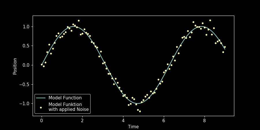
We have got a more realistic set of values by adding normal distributed random values on the model function. That’s all for now, folks!